中古マンション売買データを分析してみた(4) - 完成系の階層モデルと駅ブランド力の可視化
半年ぐらいウダウダやってましたが,今回が最終回です.自分としては満足のいく階層モデルに仕上がり,可視化までたどり着きました.ということでこれまでのエントリを別ページにまとめておきます.
問題点の修正
前回のモデルを公開したところ,@beroberoさんから以下のようにご指摘いただきました.
.@smrmkt それぐらいなら大丈夫そうです。それよりも原因わかったっぽいです。少なくともr_sのasがいらなさそうです。これがY[i]のaとバッティングして、a+asが一定の値になればいいので収束しなさそうです。よく考えるとさらに減らせる項があるかもしれません。
— berobero (@berobero11) November 11, 2014これがまさしくその通りで,項を削除することで呆気なく収束に至りました.つまり前回のモデルはこちらだったのですが,
このは駅ごとに推定する値ではなく,全物件で共通する定数なわけです.となると,下部分の駅階層モデルを,上の物件モデルにそのまま代入してあげれば,結局
と
は同じ定数項が並列しているだけということになります.具体的に代入すると,以下の形になります.
MCMCのようなシミュレーションで,定数項が今回のように2つ並列で並んでいると,2つの項の和が収束するべき値になっていれば系全体として安定するため,各々の項については永久に収束しないわけです.実際,前回のと
のtraceplotをみてもらえれば,両者が(和が一定になるように逆向きに)連動して動いているのが見て取れるかと思います*1.

モデル
モデル式
収束しない原因はわかりましたが,このを単に抜くのはいかにももったいない*2.駅の固定効果として,路線から影響を受ける項と,駅独自の効果をどちらも取得したいと考え,
としました.そして
が正規分布から生成され,その正規分布の分散が無情報事前分布になる,というモデルです.
Stanコード
前回との違いは,asがvectorとして駅ごとに推定される点,そしてasは無情報事前分布に従うパラメタs_asを分散とする正規分布にしたがう点です.その他については,基本的に前回と同じになります.
data {
    int<lower=1>            N;      # sample num
    int<lower=1>            M;      # independents' num
    int<lower=1>            N_T;    # train num
    int<lower=1>            N_S;    # station num
    matrix[N, M]            X;      # independents
    vector[N]               Y;      # dependent
    matrix[N_S, N_T]        ST;     # station-train matrix
    int<lower=1, upper=N_S> S[N];   # station
}
parameters {
    real             a;
    vector[M]        b;
    vector[N_T]      r_t;
    vector[N_S]      as;
    real             r_s[N_S];
    real<lower=0>    s;
    real<lower=0>    s_as;
    real<lower=0>    s_rs;
    real<lower=0>    s_rt;
}
model {
    # regresion model with random effect
    for (i in 1:N)
        Y[i] ~ normal(a+X[i]*b+r_s[S[i]], s);
    # prior distributions
    s ~ uniform(0, 1.0e+4);
    a ~ normal(39, 1.0e+4);
    for (i in 1:M)
        b[i] ~ normal(0, 1.0e+4);
    for (i in 1:N_S)
        r_s[i] ~ normal(as[i]+ST[i]*r_t, s_rs);
    # hierarchical prior distribution
    s_rs ~ uniform(0, 1.0e+4);
    for (i in 1:N_S)
        as[i] ~ normal(0, s_as);
    for (i in 1:N_T)
        r_t[i] ~ normal(0, s_rt);
    # 2 hierarchical prior distibution
    s_as ~ uniform(0, 1.0e+4);
    s_rt ~ uniform(0, 1.0e+4);
}
シミュレーション結果
2000回くらいイテレーションを回したら,それほど問題なく収束しました.結果はエントリの最後に載せていますが,asのパラメタが若干不安定な形での推定になってしまっています.とはいえのパラメタが大半でもあるし,まぁこんなもんかなということにしました.
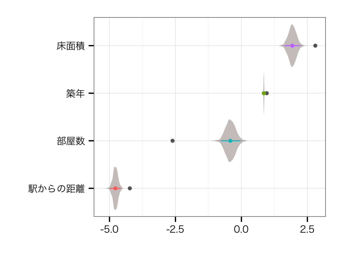
住宅レベル変数の効果
こちらの推定値は,以前の駅・路線を並列でモデルに突っ込んだときとあまり変わりません.そりゃそうですよね... もともと部屋数と床面積の相関が0.73あって,VIFも2.2程度ありました.そのことを考えたら,部屋数の効果がよりmodestなものになるのは,正しい推定ができるようになったと考えてよいのかな,と思います.
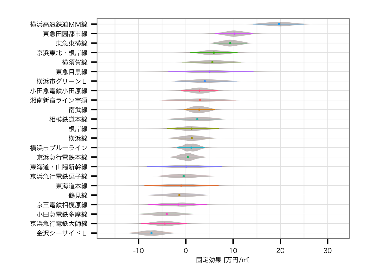
路線の効果
こちらは結構大きく結果が変わっていて,2位と3位に田園都市線,東横線という東急コンビが並びました.以前の結果だと2位が横須賀線,3位が東海道線だったことを考えると,人気の東急ブランドがキチンと評価されているこちらのほうが,妥当感が非常に強いモデルではないかなと思います*3.逆に最下位が金沢シーサイドライン*4,京急大師線,小田急多摩線とすべて主要路線の派生路線となっており,こちらも強い納得できる結果です.
駅の効果トップ10
こちらに関しては,上記モデル式のと
の2パターンについて求めました.前者は路線の影響も含んだ駅のブランド価値,後者は路線の影響を排除した純粋な駅だけのブランド価値ということになります.
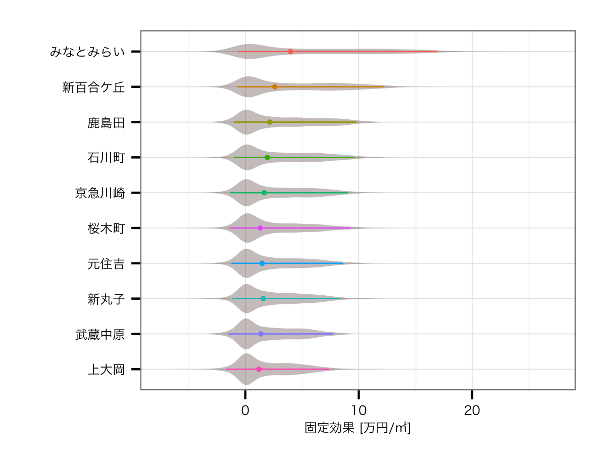
路線の影響を含んだ効果
結果はみなとみらい駅の圧勝でした.そもそもみなとみらい線自体がブランド価値No.1であるのに加えて,みなとみらい駅自体の価値がさらに高いわけですので,当然の結果といえるでしょう*5.そして2位は公示地価のエリア上昇率首都圏第1位の駅である武蔵小杉,そしてかつては横浜市の中心だった横浜駅と続きます.その下にはみなとみらい線の各駅が並び,あとは東横線,根岸線というブランド価値が高い路線の駅が並ぶ結果となりました.

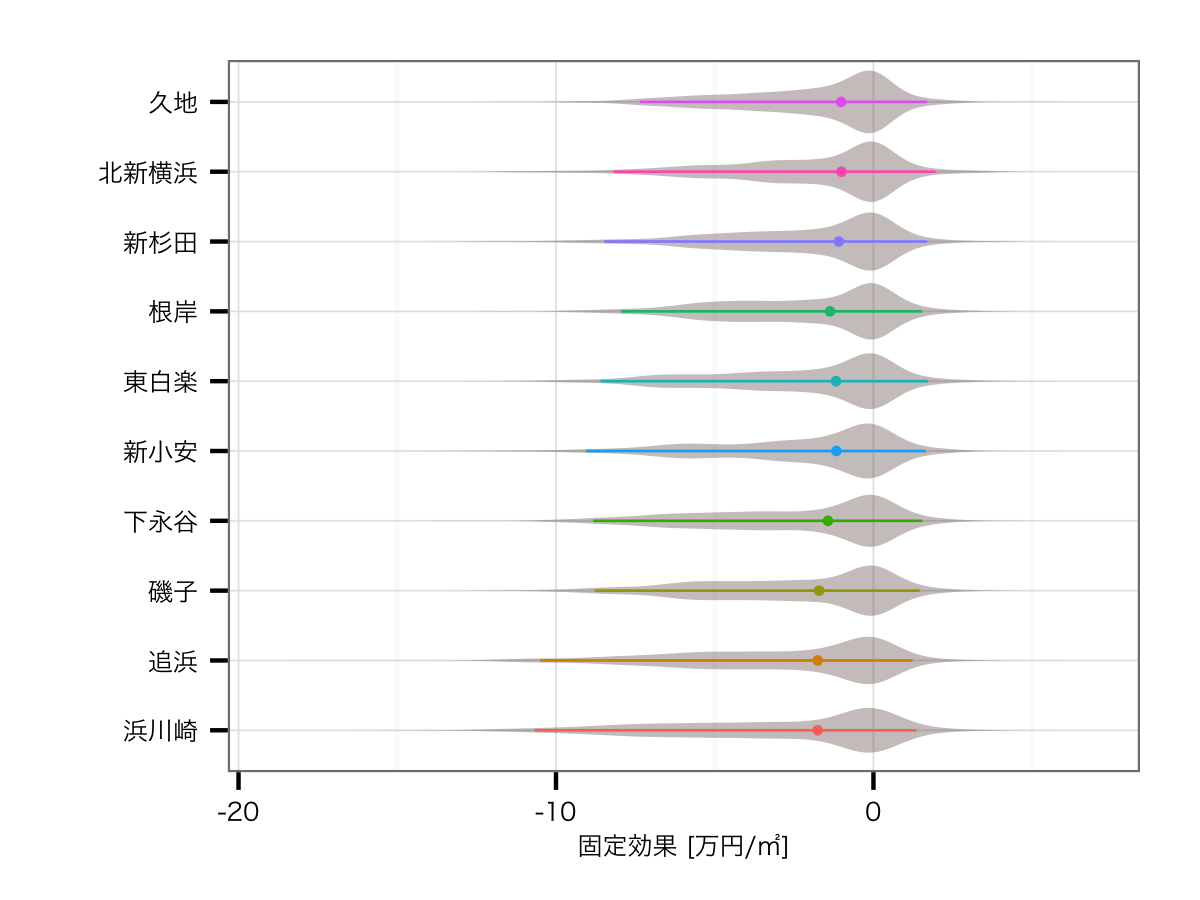
路線の影響を排除した効果
こちらはガラッと顔ぶれも分布も変わってきています.残念ながらかなり裾の長い分布になってしまっており,推定値の不安定さがそのまま分布に現れている感は否めません.とはいえ,結果自体は興味深いものとなっています.1位のみなとみらいを脇に置くと,路線効果を含んだ場合には圏外だった新百合ケ丘が2位に急浮上しています.小田急線のブランド価値がイマイチな中で,神奈川の新興高級住宅地として有名な新百合ケ丘が入っているのは,個人的にはかなり納得できます.以下は地味な南武線沿線にもかかわらずタワーマンションが乱立している鹿島田駅や,横浜屈指の高級住宅街である石川町がランクインしています.
駅の効果ワースト10
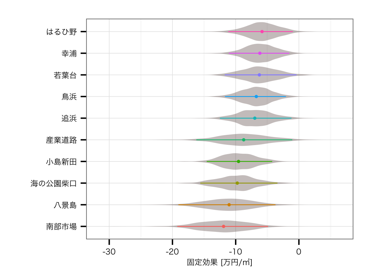
路線の影響を排除した効果
駅の影響を除くと,ワーストの方は正直ちゃんと推定できていない感があります.とはいえランクインしている駅は,どれもイマイチ目立たない駅ですね...
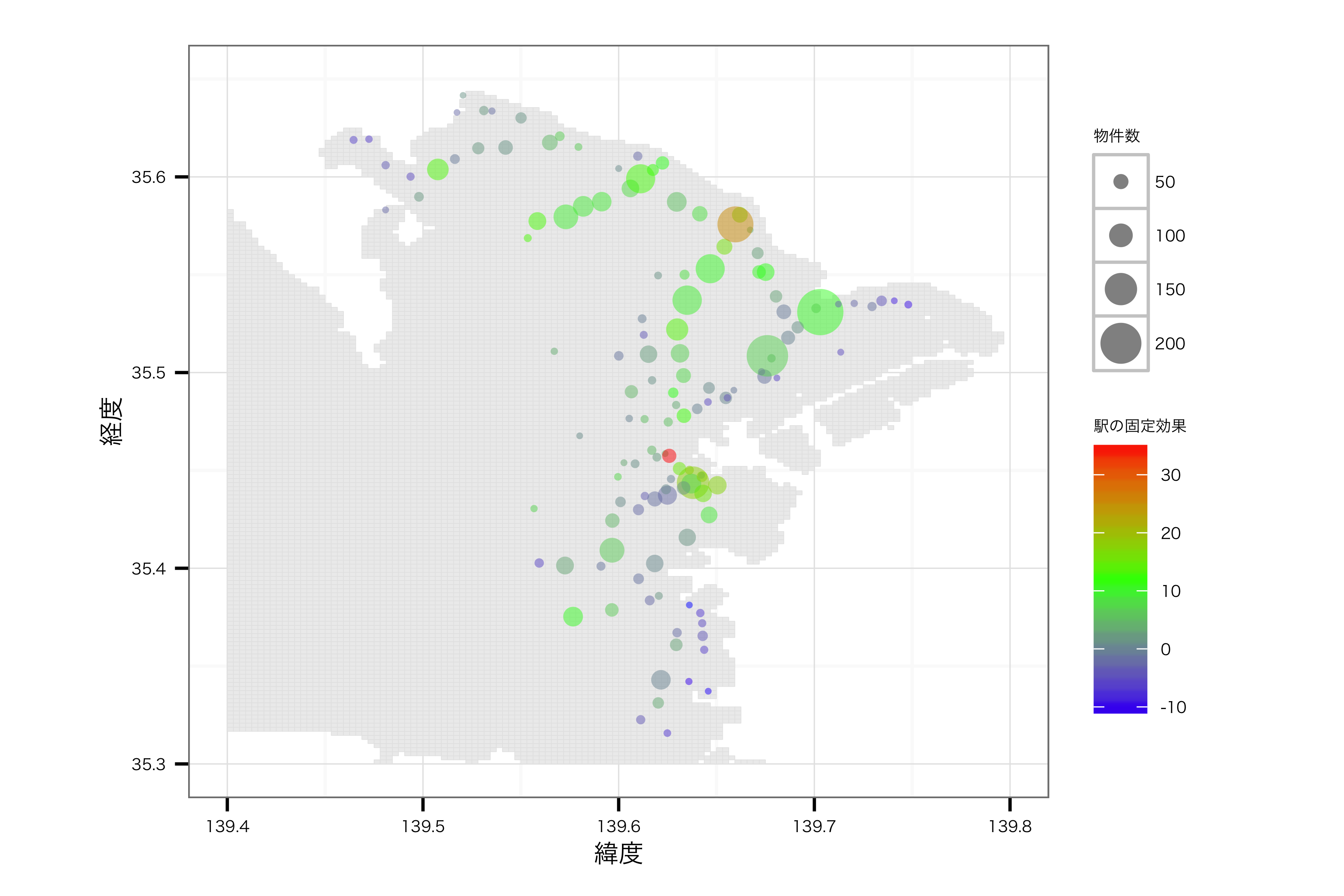
地図上にマッピング
最後に,上記の駅ごとの効果を地図上にマッピングしてみます.いつもの{ggplot2}に加えて,{maptools}, {gpclib}パッケージを使ってプロットしました.データについてはhttp://d.hatena.ne.jp/murakami_tak/20080708/p1のデータを使わせていただきました*6.また駅の緯度経度については,Geocoding APIを利用して取得しました*7.色が赤いほどプラスの効果が強く,青いほどマイナスです.そして円の大きさは制約した物件の数を表しています.

ということで
半年くらい続けてきた路線・駅の階層モデルは今回でいったん完成かなぁという形です.途中放置したりしながら,ダラダラと続けてきましたが,なんとか完成という形に持っていけてホッと一安心です.わりと試行錯誤の過程を詳細に残しているので,その点でStanやBUGSを始める方の参考になればなぁと思っています.あとはデータ数を拡充して,せめて東京県全体でやると面白い結果になるのかなぁとは思いますが,気が向いたらやるかもしれません.
コード等
Rコード
# load library
## util
library('plyr')
library('dplyr')
library('reshape2')
library('pipeR')
## stan
library('doParallel')
library('foreach')
library('rstan')
## graph
library('ggplot2')
library('maptools')
library('gpclib')

################################################################################
# Stan simulation
################################################################################

# pre-simulation
################################################################################
# load data
d = read.delim('data/mantions.csv', header=T, sep=',')
d = na.omit(d)
attach(d)
st = read.delim('data/station_train.csv', header=F, sep=',')

# package data for stan
X  = t(rbind(distance, from, room, space))
ST = st
S  = station
Y  = price
d.stan = list(N=nrow(X),
              N_T=length(unique(train)),
              N_S=length(unique(station)),
              M=ncol(X),
              X=X,
              ST=ST,
              S=S,
              Y=Y)

# simulation
################################################################################
# test procesing
if (0) {
  model.fit<-stan(file="script/2hierarchical_station_train.stan",
                  data=d.stan,
                  iter=40,
                  chains=2)
}

# parallel processing
N.chain = 3
cl = makeCluster(N.chain)
registerDoParallel(cl)
sflist = foreach(i=1:N.chain, .packages='rstan') %dopar% {
  stan(
    file='script/2hierarchical_station_train.stan',
    data=d.stan, iter=2000, thin=3,
    chains=1, chain_id=i, refresh=-1
  )
}
model.fit <- sflist2stanfit(sflist)
stopCluster(cl)

# post-simulation
################################################################################
# save data
save.image("output/2hierarchical_station_train/result.Rdata")
## get summary
print(model.fit, digits_summary=3)
fit.summary <- data.frame(summary(model.fit)$summary)
write.table(fit.summary,
            file="output/2hierarchical_station_train/fit_summary.txt",
            sep="\t",
            quote=F,
            col.names=NA)
## get plot
pdf("output/2hierarchical_station_train/fit_plot.pdf", width=600/72, height=600/72)
plot(model.fit)
dev.off()
## get traceplot
pdf("output/2hierarchical_station_train/fit_traceplot.pdf", width=600/72, height=600/72)
traceplot(model.fit)
dev.off()

# extract mcmc sample
la <- extract(model.fit, permuted = TRUE)
N.day <- nrow(d)
N.mcmc <- length(la$mu)
la$mu     #=> array
la$weight #=> matrix

################################################################################
# Draw graphs of Stan simulation result
################################################################################

# draw train distribution graph
################################################################################
## data preprocess
train_names = c('湘南新宿ライン宇須', '東海道本線', '南武線', '鶴見線', '横浜線', '根岸線',
                '横須賀線', '京浜東北・根岸線', '東急東横線', '京浜急行電鉄本線',
                '京浜急行電鉄逗子線','相模鉄道本線', '横浜市ブルーライン', '金沢シーサイドL',
                '横浜高速鉄道MM線', '横浜市グリーンL', '東海道・山陽新幹線',
                '東急目黒線', '東急田園都市線', '京王電鉄相模原線', '小田急電鉄多摩線',
                '京浜急行電鉄大師線', '小田急電鉄小田原線')
r_t = la$r_t
colnames(r_t) = train_names
r_t.melt <- melt(r_t, id = c(), value="param")
colnames(r_t.melt)[2] <- "train"
r_t.qua.melt <- ddply(r_t.melt, .(train), summarize,
                      median=median(value),
                      ymax=quantile(value, prob=0.975),
                      ymin=quantile(value, prob=0.025))
colnames(r_t.qua.melt)[2] <- "value"
r_t.melt = data.frame(r_t.melt, ymax=rep(0, nrow(r_t.melt)), ymin=rep(0, nrow(r_t.melt)))
## draw graph
p <- ggplot(r_t.melt, aes(x=reorder(train, value),
                          y=value, group=train, color=train, ymax=ymax, ymin=ymin))
p <- p + geom_violin(trim=F, fill="#5B423D", linetype="blank", alpha=I(1/3))
p <- p + geom_pointrange(data=r_t.qua.melt, size=0.20)
p <- p + coord_flip()
p <- p + labs(x="", y="固定効果 [万円/㎡]")
p <- p + theme_bw(base_family = "HiraKakuProN-W3")
p <- p + theme(axis.text.x=element_text(size=5),
               axis.title.x=element_text(size=5),
               axis.text.y=element_text(size=5),
               legend.position="none")
plot(p)
ggsave(file="output/2hierarchical_station_train/train.png",
       plot=p, dpi=300, width=4, height=3)

# draw other parameter distribution graph
################################################################################
## data preprocess
bs = data.frame(la$b)
pnames = c('駅からの距離', '築年', '部屋数', '床面積')
colnames(bs) = pnames
bs.melt <- melt(bs, id = c(), value="params")
colnames(bs.melt)[1] <- "params"
bs.qua.melt <- ddply(bs.melt, .(params), summarize,
                     median=median(value),
                     ymax=quantile(value, prob=0.975),
                     ymin=quantile(value, prob=0.025))
colnames(bs.qua.melt)[2] <- "value"
bs.melt = data.frame(bs.melt, ymax=rep(0, nrow(bs.melt)), ymin=rep(0, nrow(bs.melt)))
bs.lm <- data.frame(params=pnames,
                    value=c(-4.23, 0.96, -2.61, 2.80), ymax=rep(0, 4), ymin=rep(0, 4))
## draw graph
p <- ggplot(bs.melt, aes(x=reorder(params, value),
                         y=value, group=params, color=params, ymax=ymax, ymin=ymin))
p <- p + geom_point(data=bs.lm, color="black", size=1.6, alpha=I(2/3))
p <- p + geom_violin(trim=F, fill="#5B423D", scale="width", linetype="blank", alpha=I(1/3))
p <- p + geom_pointrange(data=bs.qua.melt, size=0.40)
p <- p + coord_flip()
p <- p + labs(x="", y="")
p <- p + theme_bw(base_family = "HiraKakuProN-W3")
p <- p + theme(axis.text.x=element_text(size=8),
               axis.title.x=element_text(size=8),
               axis.text.y=element_text(size=8),
               legend.position="none")
plot(p)
ggsave(file="output/2hierarchical_station_train/params.png",
       plot=p, dpi=300, width=4, height=3)

# draw station(price higher) full distribution graph
################################################################################
station_names = c('みなとみらい', '武蔵小杉', '横浜', '日本大通り', '馬車道',
                  '元町・中華街', '新丸子', '元住吉', '石川町', '桜木町')
r_s = la$r_s[, c(128, 109, 19, 125, 87, 129, 62, 47, 79, 70)]
colnames(r_s) = station_names
r_s.melt <- melt(r_s, id = c(), value="param")
colnames(r_s.melt)[2] <- "station"
r_s.qua.melt <- ddply(r_s.melt, .(station), summarize,
                      median=median(value),
                      ymax=quantile(value, prob=0.975),
                      ymin=quantile(value, prob=0.025))
colnames(r_s.qua.melt)[2] <- "value"
r_s.melt = data.frame(r_s.melt, ymax=rep(0, nrow(r_s.melt)), ymin=rep(0, nrow(r_s.melt)))
## draw graph
p <- ggplot(r_s.melt, aes(x=reorder(station, value),
                          y=value, group=station, color=station, ymax=ymax, ymin=ymin))
p <- p + geom_violin(trim=F, fill="#5B423D", linetype="blank", alpha=I(1/3))
p <- p + geom_pointrange(data=r_s.qua.melt, size=0.30)
p <- p + coord_flip()
p <- p + labs(x="", y="固定効果 [万円/㎡]")
p <- p + theme_bw(base_family = "HiraKakuProN-W3")
p <- p + theme(axis.text.x=element_text(size=6),
               axis.title.x=element_text(size=6),
               axis.text.y=element_text(size=6),
               legend.position="none")
plot(p)
ggsave(file="output/2hierarchical_station_train/station_full_high.png",
       plot=p, dpi=300, width=4, height=3)

# draw station(price lower) full distribution graph
################################################################################
station_names = c('南部市場', '八景島', '海の公園柴口', '小島新田', '産業道路',
                  '追浜', '鳥浜', '若葉台', '幸浦', 'はるひ野')
r_s = la$r_s[, c(101, 49, 130, 102, 112, 31, 35, 83, 11, 92)]
colnames(r_s) = station_names
r_s.melt <- melt(r_s, id = c(), value="param")
colnames(r_s.melt)[2] <- "station"
r_s.qua.melt <- ddply(r_s.melt, .(station), summarize,
                      median=median(value),
                      ymax=quantile(value, prob=0.975),
                      ymin=quantile(value, prob=0.025))
colnames(r_s.qua.melt)[2] <- "value"
r_s.melt = data.frame(r_s.melt, ymax=rep(0, nrow(r_s.melt)), ymin=rep(0, nrow(r_s.melt)))
## draw graph
p <- ggplot(r_s.melt, aes(x=reorder(station, value),
                          y=value, group=station, color=station, ymax=ymax, ymin=ymin))
p <- p + geom_violin(trim=F, fill="#5B423D", linetype="blank", alpha=I(1/3))
p <- p + geom_pointrange(data=r_s.qua.melt, size=0.30)
p <- p + coord_flip()
p <- p + labs(x="", y="固定効果 [万円/㎡]")
p <- p + theme_bw(base_family = "HiraKakuProN-W3")
p <- p + theme(axis.text.x=element_text(size=6),
               axis.title.x=element_text(size=6),
               axis.text.y=element_text(size=6),
               legend.position="none")
plot(p)
ggsave(file="output/2hierarchical_station_train/station_full_low.png",
       plot=p, dpi=300, width=4, height=3)

# draw station(price higher) specific distribution graph
################################################################################
station_names = c('みなとみらい', '新百合ケ丘', '鹿島田', '石川町', '京急川崎',
                  '新丸子', '元住吉', '武蔵中原', '桜木町', '上大岡')
as = la$as[, c(128, 124, 89, 79, 97, 62, 47, 108, 70, 40)]
colnames(as) = station_names
as.melt <- melt(as, id = c(), value="param")
colnames(as.melt)[2] <- "station"
as.qua.melt <- ddply(as.melt, .(station), summarize,
                      median=median(value),
                      ymax=quantile(value, prob=0.975),
                      ymin=quantile(value, prob=0.025))
colnames(as.qua.melt)[2] <- "value"
as.melt = data.frame(as.melt, ymax=rep(0, nrow(as.melt)), ymin=rep(0, nrow(as.melt)))
## draw graph
p <- ggplot(as.melt, aes(x=reorder(station, value),
                          y=value, group=station, color=station, ymax=ymax, ymin=ymin))
p <- p + geom_violin(trim=F, fill="#5B423D", linetype="blank", alpha=I(1/3))
p <- p + geom_pointrange(data=as.qua.melt, size=0.30)
p <- p + coord_flip()
p <- p + labs(x="", y="固定効果 [万円/㎡]")
p <- p + theme_bw(base_family = "HiraKakuProN-W3")
p <- p + theme(axis.text.x=element_text(size=6),
               axis.title.x=element_text(size=6),
               axis.text.y=element_text(size=6),
               legend.position="none")
plot(p)
ggsave(file="output/2hierarchical_station_train/station_specific_high.png",
       plot=p, dpi=300, width=4, height=3)

# draw station(price lower) specific distribution graph
################################################################################
station_names = c('浜川崎', '追浜', '磯子', '下永谷', '根岸',
                  '東白楽', '新小安', '新杉田', '久地', '北新横浜')
as = la$as[, c(74, 31, 27, 43, 18, 68, 63, 65, 1, 100)]
colnames(as) = station_names
as.melt <- melt(as, id = c(), value="param")
colnames(as.melt)[2] <- "station"
as.qua.melt <- ddply(as.melt, .(station), summarize,
                      median=median(value),
                      ymax=quantile(value, prob=0.975),
                      ymin=quantile(value, prob=0.025))
colnames(as.qua.melt)[2] <- "value"
as.melt = data.frame(as.melt, ymax=rep(0, nrow(as.melt)), ymin=rep(0, nrow(as.melt)))
## draw graph
p <- ggplot(as.melt, aes(x=reorder(station, value),
                          y=value, group=station, color=station, ymax=ymax, ymin=ymin))
p <- p + geom_violin(trim=F, fill="#5B423D", linetype="blank", alpha=I(1/3))
p <- p + geom_pointrange(data=as.qua.melt, size=0.30)
p <- p + coord_flip()
p <- p + labs(x="", y="固定効果 [万円/㎡]")
p <- p + theme_bw(base_family = "HiraKakuProN-W3")
p <- p + theme(axis.text.x=element_text(size=6),
               axis.title.x=element_text(size=6),
               axis.text.y=element_text(size=6),
               legend.position="none")
plot(p)
ggsave(file="output/2hierarchical_station_train/station_specific_low.png",
       plot=p, dpi=300, width=4, height=3)

################################################################################
# Draw geo graphs using maptools
################################################################################

# preprocessing
################################################################################
# load geo map data
#kanagawa = readShapePoly('data/mesh03-tky-14-shp/mesh03-tky-14.shp')
kanagawa <- readShapePoly("data/mesh05-jgd-14-shp/mesh05-jgd-14.shp")
gpclibPermit()
df = fortify(kanagawa)

# load mantion and location data
locations = read.csv('data/locations.tsv')
mantions = read.csv('data/mantions.csv')

# samples grouped by station
mantions.grouped = summarise(group_by(mantions, station), n())
colnames(mantions.grouped)[2] = 'n'

# draw geo map with station full effect
################################################################################
# acquire fixed effect
hmc_samples = melt(la$r_s)
colnames(hmc_samples)[2] = 'station'
hmc_samples.grouped = summarise(group_by(hmc_samples, station),
                                mean(value), sd(value))
colnames(hmc_samples.grouped)[2:3] = c('effect', 'effect_sd')

# join data
geo_data = merge(merge(locations, mantions.grouped), hmc_samples.grouped)

# plot
p = ggplot(df)
p = p + geom_polygon(
  aes(long, lat, group=group),
  colour='gray90', fill='gray93', size=0.1
)
p = p + xlim(c(139.40, 139.80)) + ylim(c(35.30, 35.65))
p = p + coord_equal()
p = p + geom_point(
  data=geo_data, alpha=0.5,
  aes(x=long, y=lat, colour=effect, size=n)
)
p = p + scale_color_gradientn(colours=c('blue', 'green', 'red'))
p = p + scale_size_continuous(range=c(1, 7))
p <- p + theme_bw(base_family = "HiraKakuProN-W3")
p <- p + theme(axis.text.x=element_text(size=5),
               axis.title.x=element_text(size=8),
               axis.text.y=element_text(size=5),
               axis.title.y=element_text(size=8),
               legend.title=element_text(size=5),
               legend.text=element_text(size=5))
p <- p + labs(x='緯度', y='経度', colour='駅の固定効果', size='物件数')
p <- p + theme(
  panel.background = element_rect(
    fill = "white", colour = "black",
    size= 0.2 , linetype = 1
  )
)
plot(p)
ggsave(file='output/2hierarchical_station_train/geo_mapping_full.png',
       plot=p, dpi=600, width=6, height=4)

# draw geo map with station specific effect
################################################################################
# acquire fixed effect
hmc_samples = melt(la$as)
colnames(hmc_samples)[2] = 'station'
hmc_samples.grouped = summarise(group_by(hmc_samples, station),
                                mean(value), sd(value))
colnames(hmc_samples.grouped)[2:3] = c('effect', 'effect_sd')

# join data
geo_data = merge(merge(locations, mantions.grouped), hmc_samples.grouped)

# plot
p = ggplot(df)
p = p + geom_polygon(
  aes(long, lat, group=group),
  colour='gray90', fill='gray93', size=0.1
)
p = p + xlim(c(139.40, 139.80)) + ylim(c(35.30, 35.65))
p = p + coord_equal()
p = p + geom_point(
  data=geo_data, alpha=0.5,
  aes(x=long, y=lat, colour=effect, size=n)
)
p = p + scale_color_gradientn(colours=c('blue', 'green', 'red'))
p = p + scale_size_continuous(range=c(1, 7))
p <- p + theme_bw(base_family = "HiraKakuProN-W3")
p <- p + theme(axis.text.x=element_text(size=5),
               axis.title.x=element_text(size=8),
               axis.text.y=element_text(size=5),
               axis.title.y=element_text(size=8),
               legend.title=element_text(size=5),
               legend.text=element_text(size=5))
p <- p + labs(x='緯度', y='経度', colour='駅の固定効果', size='物件数')
p <- p + theme(
  panel.background = element_rect(
    fill = "white", colour = "black",
    size= 0.2 , linetype = 1
  )
)
plot(p)
ggsave(file='output/2hierarchical_station_train/geo_mapping_specific.png',
       plot=p, dpi=600, width=6, height=4)
Stanコード
data {
    int<lower=1>            N;      # sample num
    int<lower=1>            M;      # independents' num
    int<lower=1>            N_T;    # train num
    int<lower=1>            N_S;    # station num
    matrix[N, M]            X;      # independents
    vector[N]               Y;      # dependent
    matrix[N_S, N_T]        ST;     # station-train matrix
    int<lower=1, upper=N_S> S[N];   # station
}
parameters {
    real             a;
    vector[M]        b;
    vector[N_T]      r_t;
    vector[N_S]      as;
    real             r_s[N_S];
    real<lower=0>    s;
    real<lower=0>    s_as;
    real<lower=0>    s_rs;
    real<lower=0>    s_rt;
}
model {
    # regresion model with random effect
    for (i in 1:N)
        Y[i] ~ normal(a+X[i]*b+r_s[S[i]], s);
    # prior distributions
    s ~ uniform(0, 1.0e+4);
    a ~ normal(39, 1.0e+4);
    for (i in 1:M)
        b[i] ~ normal(0, 1.0e+4);
    for (i in 1:N_S)
        r_s[i] ~ normal(as[i]+ST[i]*r_t, s_rs);
    # hierarchical prior distribution
    s_rs ~ uniform(0, 1.0e+4);
    for (i in 1:N_S)
        as[i] ~ normal(0, s_as);
    for (i in 1:N_T)
        r_t[i] ~ normal(0, s_rt);
    # 2 hierarchical prior distibution
    s_as ~ uniform(0, 1.0e+4);
    s_rt ~ uniform(0, 1.0e+4);
}
推定値のサマリ
> print(model.fit, digits_summary=3) Inference for Stan model: 2hierarchical_station_train. 3 chains, each with iter=2000; warmup=1000; thin=3; post-warmup draws per chain=334, total post-warmup draws=1002. mean se_mean sd 2.5% 25% 50% 75% 97.5% n_eff Rhat a -1658.141 0.691 21.118 -1701.536 -1672.255 -1658.249 -1643.501 -1615.856 935 1.001 b[1] -4.777 0.003 0.096 -4.966 -4.840 -4.778 -4.713 -4.584 1002 1.000 b[2] 0.850 0.000 0.011 0.829 0.843 0.850 0.857 0.871 945 1.000 b[3] -0.415 0.006 0.191 -0.778 -0.538 -0.420 -0.288 -0.035 1002 0.998 b[4] 1.930 0.005 0.149 1.642 1.833 1.927 2.030 2.227 1002 0.999 r_t[1] 2.879 0.212 4.119 -5.035 0.154 3.005 5.720 10.592 379 1.002 r_t[2] -0.979 0.205 4.102 -8.763 -3.925 -1.007 1.762 6.918 400 1.001 r_t[3] 2.852 0.235 1.690 -0.311 1.638 2.805 3.977 6.131 52 1.019 r_t[4] -1.413 0.136 3.208 -7.988 -3.523 -1.369 0.831 4.392 555 1.004 r_t[5] 1.303 0.111 2.244 -3.123 -0.236 1.239 2.773 5.869 411 1.003 r_t[6] 1.321 0.105 2.822 -3.948 -0.585 1.230 3.181 6.947 721 1.002 r_t[7] 5.506 0.114 3.176 -0.793 3.381 5.611 7.673 11.619 776 1.003 r_t[8] 5.961 0.131 2.609 0.923 4.178 5.933 7.800 10.932 399 1.002 r_t[9] 9.417 0.258 1.880 5.846 8.124 9.403 10.703 13.011 53 1.021 r_t[10] 0.379 0.255 1.606 -2.665 -0.758 0.395 1.401 3.589 40 1.031 r_t[11] -0.473 0.129 3.141 -7.037 -2.602 -0.475 1.511 5.740 590 1.002 r_t[12] 2.369 0.179 2.904 -3.219 0.324 2.424 4.486 7.726 263 1.008 r_t[13] 1.082 0.166 1.539 -1.898 0.038 1.136 2.140 3.966 86 1.014 r_t[14] -7.283 0.202 2.293 -11.900 -8.809 -7.274 -5.714 -2.750 128 1.009 r_t[15] 19.689 0.271 2.815 14.148 17.764 19.725 21.553 25.002 108 1.014 r_t[16] 4.080 0.188 3.423 -2.346 1.806 3.987 6.308 10.849 333 1.002 r_t[17] 0.003 0.140 4.136 -8.208 -2.796 0.071 2.857 7.643 871 0.999 r_t[18] 4.971 0.157 4.612 -3.735 1.754 5.023 7.970 14.311 866 1.001 r_t[19] 10.298 0.265 2.078 6.166 8.906 10.314 11.763 14.124 62 1.021 r_t[20] -1.777 0.189 3.148 -7.955 -3.871 -1.600 0.361 4.539 278 1.011 r_t[21] -4.138 0.172 2.928 -10.026 -6.069 -4.058 -2.188 1.618 290 1.019 r_t[22] -4.442 0.206 2.487 -9.489 -6.005 -4.449 -2.828 0.303 146 1.015 r_t[23] 2.882 0.223 2.100 -1.060 1.490 2.892 4.318 6.888 89 1.021 as[1] -1.833 0.539 2.477 -7.361 -3.416 -1.020 -0.037 1.688 21 1.205 as[2] -1.260 0.375 2.545 -7.551 -2.547 -0.460 0.148 2.785 46 1.083 as[3] -1.400 0.398 2.313 -6.739 -2.883 -0.672 0.053 2.306 34 1.119 as[4] -0.134 0.069 1.920 -4.492 -1.032 -0.026 0.870 3.728 785 1.016 as[5] -1.961 0.557 2.731 -8.224 -3.657 -0.999 0.005 2.115 24 1.180 as[6] -1.053 0.331 2.241 -6.604 -2.265 -0.323 0.169 2.821 46 1.082 as[7] -1.328 0.383 2.105 -6.051 -2.582 -0.672 0.075 1.901 30 1.143 as[8] 0.655 0.133 1.974 -3.035 -0.280 0.230 1.687 4.961 221 1.024 as[9] 0.904 0.161 2.461 -3.315 -0.267 0.269 2.044 6.915 233 1.040 as[10] -0.137 0.058 1.770 -4.002 -0.990 -0.028 0.741 3.291 936 1.003 as[11] 0.410 0.066 2.082 -3.915 -0.501 0.130 1.475 5.031 1002 1.008 as[12] 0.719 0.127 1.837 -2.515 -0.227 0.255 1.775 4.978 209 1.041 as[13] -0.532 0.097 1.894 -4.793 -1.580 -0.207 0.392 3.124 385 1.017 as[14] 0.339 0.055 1.756 -3.138 -0.487 0.068 1.223 4.241 1002 1.006 as[15] -0.924 0.271 2.018 -5.467 -2.064 -0.326 0.199 2.916 56 1.062 as[16] -0.379 0.063 1.998 -4.707 -1.248 -0.105 0.424 3.729 1002 1.009 as[17] 0.260 0.067 2.121 -4.062 -0.639 0.077 1.288 5.203 1002 1.004 as[18] -2.081 0.611 2.625 -7.953 -4.012 -1.368 -0.021 1.538 18 1.251 as[19] -1.013 0.244 2.685 -7.401 -2.295 -0.253 0.250 3.740 121 1.053 as[20] 0.266 0.079 2.494 -4.810 -0.746 0.048 1.141 6.214 1002 1.005 as[21] 0.601 0.151 2.563 -3.769 -0.549 0.085 1.577 7.037 288 1.019 as[22] -0.470 0.092 1.863 -4.520 -1.456 -0.132 0.414 3.116 410 1.021 as[23] -0.654 0.087 1.814 -4.774 -1.617 -0.253 0.285 2.482 435 1.024 as[24] 0.435 0.077 2.072 -3.463 -0.539 0.085 1.304 5.692 725 1.016 as[25] 0.682 0.135 1.898 -2.757 -0.257 0.314 1.713 5.005 197 1.033 as[26] 0.113 0.060 1.900 -4.082 -0.745 0.067 0.966 4.206 1002 1.001 as[27] -2.455 0.715 2.907 -8.786 -4.621 -1.711 -0.029 1.459 17 1.291 as[28] 0.030 0.054 1.695 -3.608 -0.801 0.008 0.837 3.688 1002 0.999 as[29] -1.452 0.420 2.464 -7.655 -2.854 -0.576 0.116 2.235 34 1.139 as[30] -1.220 0.350 2.119 -6.306 -2.486 -0.567 0.126 1.975 37 1.105 as[31] -2.798 0.791 3.245 -10.502 -5.095 -1.756 -0.113 1.233 17 1.287 as[32] -0.286 0.078 1.890 -4.399 -1.078 -0.110 0.612 3.623 581 1.008 as[33] 0.586 0.082 1.898 -3.062 -0.386 0.170 1.575 5.121 538 1.028 as[34] -1.023 0.230 2.362 -6.882 -2.237 -0.351 0.220 2.956 106 1.057 as[35] 0.231 0.061 1.837 -3.702 -0.558 0.100 1.128 3.987 897 1.000 as[36] 0.916 0.218 2.250 -2.879 -0.253 0.314 2.145 6.202 106 1.048 as[37] -1.966 0.555 2.874 -8.873 -3.577 -0.964 -0.002 1.998 27 1.155 as[38] 0.860 0.242 2.305 -3.141 -0.270 0.289 1.971 6.234 91 1.040 as[39] -0.298 0.056 1.758 -4.143 -1.147 -0.073 0.435 3.261 1002 1.010 as[40] 1.939 0.594 2.544 -1.722 0.035 1.198 3.769 7.406 18 1.247 as[41] -0.487 0.082 2.349 -6.092 -1.647 -0.127 0.520 4.426 829 1.009 as[42] 0.713 0.133 1.757 -2.605 -0.187 0.292 1.683 4.689 174 1.048 as[43] -2.394 0.713 2.931 -8.829 -4.577 -1.433 -0.042 1.541 17 1.264 as[44] 0.799 0.184 2.160 -3.346 -0.264 0.270 1.971 5.725 138 1.049 as[45] -0.483 0.065 1.912 -4.738 -1.453 -0.144 0.378 3.014 871 1.023 as[46] -0.268 0.074 2.143 -5.247 -1.180 -0.045 0.700 3.968 845 1.006 as[47] 2.376 0.682 2.847 -1.227 0.050 1.482 4.525 8.636 17 1.265 as[48] -0.598 0.108 1.918 -4.869 -1.612 -0.169 0.342 3.010 315 1.028 as[49] -1.477 0.412 2.740 -8.362 -2.795 -0.461 0.138 2.566 44 1.087 as[50] -1.420 0.386 2.251 -6.476 -2.783 -0.724 0.032 2.152 34 1.123 as[51] -1.001 0.297 1.987 -5.398 -2.271 -0.469 0.129 2.305 45 1.080 as[52] 0.471 0.079 2.496 -4.310 -0.523 0.094 1.505 6.757 1002 1.008 as[53] 1.445 0.398 2.227 -1.895 -0.065 0.836 2.800 6.752 31 1.120 as[54] 0.286 0.089 2.346 -4.391 -0.680 0.073 1.303 5.738 689 1.002 as[55] -0.694 0.210 1.869 -5.196 -1.639 -0.248 0.212 2.797 79 1.050 as[56] -0.388 0.065 1.745 -4.179 -1.329 -0.158 0.412 3.086 719 1.006 as[57] -0.395 0.064 1.760 -4.087 -1.381 -0.142 0.425 3.352 762 1.008 as[58] 1.319 0.380 2.497 -2.641 -0.127 0.473 2.673 7.543 43 1.097 as[59] -0.668 0.091 1.800 -4.845 -1.584 -0.245 0.244 2.737 392 1.031 as[60] 0.882 0.149 2.325 -3.209 -0.333 0.277 2.104 6.314 243 1.041 as[61] 1.217 0.363 2.168 -2.327 -0.110 0.571 2.511 6.158 36 1.101 as[62] 2.375 0.662 2.760 -1.185 0.071 1.579 4.310 8.370 17 1.289 as[63] -2.189 0.619 2.872 -9.049 -3.864 -1.169 -0.050 1.645 22 1.192 as[64] 0.755 0.149 2.432 -3.565 -0.375 0.210 1.934 6.602 267 1.024 as[65] -2.006 0.587 2.700 -8.473 -3.686 -1.090 0.006 1.698 21 1.210 as[66] 0.030 0.082 2.401 -5.173 -0.931 0.030 1.046 5.106 853 0.998 as[67] 0.694 0.107 2.474 -4.240 -0.440 0.152 1.864 6.366 530 1.021 as[68] -2.148 0.609 2.822 -8.597 -3.967 -1.178 0.006 1.720 21 1.205 as[69] 0.038 0.064 1.856 -3.949 -0.740 0.027 0.919 3.869 844 1.002 as[70] 2.424 0.697 2.995 -1.398 0.085 1.312 4.475 9.321 18 1.246 as[71] -0.796 0.211 1.859 -4.803 -1.893 -0.388 0.191 2.508 78 1.052 as[72] -0.314 0.058 1.841 -4.501 -1.155 -0.113 0.498 3.500 1002 1.007 as[73] -0.826 0.198 2.341 -6.814 -1.821 -0.191 0.234 3.230 140 1.032 as[74] -2.964 0.845 3.490 -10.673 -5.470 -1.756 -0.086 1.353 17 1.269 as[75] 1.194 0.343 2.136 -2.240 -0.098 0.514 2.504 5.921 39 1.106 as[76] 0.931 0.272 1.872 -2.280 -0.144 0.361 2.047 5.242 47 1.089 as[77] 1.392 0.380 2.158 -2.134 -0.048 0.700 2.833 6.167 32 1.136 as[78] -0.622 0.092 2.550 -6.574 -1.709 -0.131 0.484 4.554 765 1.012 as[79] 2.938 0.822 3.191 -0.992 0.134 1.948 5.499 9.645 15 1.337 as[80] 1.052 0.299 2.473 -3.097 -0.262 0.275 2.297 6.961 68 1.053 as[81] -1.571 0.464 2.538 -7.859 -2.938 -0.672 0.058 2.027 30 1.148 as[82] 1.069 0.312 1.896 -2.066 -0.094 0.545 2.235 5.601 37 1.121 as[83] -1.726 0.521 2.725 -8.211 -3.132 -0.733 0.045 1.956 27 1.148 as[84] -0.394 0.083 2.066 -5.285 -1.343 -0.146 0.503 4.093 626 1.011 as[85] 0.791 0.165 2.267 -3.218 -0.310 0.238 1.803 6.257 190 1.031 as[86] -1.166 0.363 2.095 -5.891 -2.515 -0.472 0.112 2.506 33 1.123 as[87] -0.776 0.195 2.075 -5.772 -1.745 -0.287 0.298 2.847 113 1.045 as[88] 1.181 0.305 2.519 -2.818 -0.168 0.353 2.545 7.378 68 1.070 as[89] 3.047 0.870 3.319 -1.032 0.098 2.156 5.641 9.804 15 1.358 as[90] 0.092 0.058 1.784 -3.708 -0.751 0.015 0.948 3.865 959 1.001 as[91] 0.921 0.281 2.127 -2.453 -0.238 0.331 2.087 5.785 57 1.057 as[92] -0.725 0.127 2.299 -6.265 -1.690 -0.179 0.324 3.272 330 1.033 as[93] 1.240 0.345 2.217 -2.193 -0.121 0.547 2.483 6.547 41 1.089 as[94] 0.207 0.058 1.824 -3.675 -0.613 0.050 1.040 4.093 1002 1.004 as[95] 0.137 0.057 1.790 -3.632 -0.682 0.036 0.931 4.023 1002 1.005 as[96] -0.879 0.228 2.042 -5.681 -1.995 -0.262 0.214 2.836 80 1.052 as[97] 2.627 0.763 3.053 -1.320 0.042 1.663 5.046 9.085 16 1.317 as[98] 1.952 0.585 2.568 -1.548 0.013 1.014 3.713 7.843 19 1.228 as[99] -0.443 0.085 2.294 -5.606 -1.569 -0.112 0.679 4.117 724 1.010 as[100] -1.892 0.536 2.682 -8.201 -3.400 -1.007 0.007 1.956 25 1.174 as[101] -1.645 0.468 2.760 -7.969 -3.033 -0.660 0.088 2.622 35 1.127 as[102] -1.867 0.532 2.664 -8.170 -3.465 -0.865 0.026 1.772 25 1.172 as[103] 0.075 0.062 1.905 -3.707 -0.717 0.017 0.880 4.628 953 1.003 as[104] 1.118 0.245 2.263 -2.596 -0.162 0.421 2.305 6.141 85 1.076 as[105] -0.043 0.060 1.826 -3.727 -0.949 -0.017 0.826 3.953 928 0.998 as[106] 1.713 0.469 2.724 -2.349 -0.076 0.881 3.239 8.216 34 1.120 as[107] 1.902 0.513 2.689 -1.935 0.006 0.957 3.536 8.221 28 1.161 as[108] 2.094 0.579 2.596 -1.493 -0.002 1.373 4.162 7.713 20 1.222 as[109] 0.901 0.202 2.684 -4.321 -0.316 0.257 2.044 7.270 177 1.044 as[110] 1.104 0.306 2.027 -2.217 -0.146 0.505 2.316 5.481 44 1.080 as[111] -0.827 0.178 1.988 -5.443 -1.841 -0.302 0.210 2.691 125 1.048 as[112] -1.564 0.492 2.767 -8.030 -3.080 -0.575 0.105 2.687 32 1.134 as[113] -1.255 0.358 2.257 -6.735 -2.467 -0.558 0.121 2.246 40 1.099 as[114] -0.113 0.069 2.175 -4.568 -1.147 -0.029 0.804 4.990 1002 1.003 as[115] 1.464 0.436 2.611 -2.781 -0.116 0.636 2.915 7.512 36 1.114 as[116] -0.082 0.051 1.602 -3.356 -0.914 -0.031 0.691 3.402 998 1.000 as[117] -1.495 0.439 2.716 -8.526 -2.718 -0.559 0.106 2.757 38 1.103 as[118] -0.080 0.055 1.736 -3.945 -0.895 -0.023 0.829 3.244 1002 0.999 as[119] -0.318 0.066 2.091 -5.798 -1.178 -0.081 0.570 3.729 1002 1.011 as[120] 1.564 0.466 2.419 -2.140 -0.044 0.748 3.081 6.978 27 1.151 as[121] -1.675 0.484 2.642 -7.745 -3.137 -0.802 0.044 2.298 30 1.129 as[122] 1.329 0.356 2.486 -2.577 -0.127 0.439 2.729 7.291 49 1.076 as[123] 0.739 0.108 1.840 -2.709 -0.156 0.356 1.762 4.859 288 1.035 as[124] 3.915 1.094 4.073 -0.704 0.205 2.600 7.269 12.255 14 1.391 as[125] -0.717 0.166 2.056 -5.373 -1.827 -0.251 0.236 3.328 153 1.028 as[126] -0.091 0.058 1.823 -3.983 -1.008 -0.025 0.754 3.718 1002 0.999 as[127] 1.006 0.296 2.033 -2.841 -0.132 0.410 2.210 5.793 47 1.073 as[128] 5.662 1.597 5.666 -0.624 0.290 3.985 10.412 16.942 13 1.427 as[129] -0.893 0.173 2.193 -6.070 -2.040 -0.307 0.231 3.074 160 1.048 as[130] -1.042 0.307 2.365 -7.006 -2.135 -0.315 0.211 3.047 59 1.068 as[131] -0.334 0.063 1.815 -4.550 -1.170 -0.119 0.558 3.214 833 1.007 as[132] 0.285 0.055 1.681 -3.321 -0.403 0.124 1.096 3.681 934 1.004 as[133] -0.118 0.077 2.423 -5.575 -1.162 -0.016 0.790 5.226 1002 0.999 r_s[1] -2.249 0.336 2.211 -6.410 -3.821 -2.263 -0.731 2.113 43 1.036 r_s[2] -3.914 0.225 2.238 -8.387 -5.455 -3.870 -2.391 0.306 99 1.022 r_s[3] 5.639 0.307 2.223 1.271 4.089 5.591 7.150 10.038 53 1.026 r_s[4] 0.713 0.254 1.793 -2.683 -0.563 0.731 1.929 4.177 50 1.026 r_s[5] -5.278 0.243 2.698 -10.429 -7.131 -5.259 -3.487 -0.139 123 1.016 r_s[6] -1.250 0.273 2.140 -5.280 -2.644 -1.240 0.199 2.980 62 1.015 r_s[7] -0.617 0.296 1.765 -3.927 -1.868 -0.636 0.604 2.666 36 1.034 r_s[8] 9.091 0.274 1.665 5.943 7.921 9.042 10.224 12.440 37 1.037 r_s[9] 10.436 0.290 1.499 7.530 9.286 10.455 11.529 13.214 27 1.053 r_s[10] 2.710 0.265 1.821 -0.613 1.388 2.661 4.006 6.317 47 1.028 r_s[11] -6.141 0.223 2.433 -11.083 -7.757 -6.180 -4.561 -1.518 119 1.018 r_s[12] 2.309 0.305 2.293 -2.359 0.854 2.290 3.782 7.114 57 1.022 r_s[13] -0.244 0.235 2.260 -4.609 -1.765 -0.252 1.292 4.283 93 1.020 r_s[14] 10.361 0.288 1.536 7.486 9.291 10.363 11.440 13.219 28 1.050 r_s[15] -2.165 0.284 2.041 -6.288 -3.438 -2.181 -0.838 1.905 51 1.026 r_s[16] 1.863 0.298 2.179 -2.327 0.360 1.776 3.364 6.154 53 1.023 r_s[17] -3.588 0.311 2.460 -8.283 -5.193 -3.549 -1.867 1.226 63 1.024 r_s[18] 1.698 0.308 1.701 -1.518 0.464 1.706 2.856 4.996 30 1.052 r_s[19] 17.952 0.280 1.545 15.073 16.807 17.882 19.053 20.943 30 1.042 r_s[20] -0.566 0.185 3.899 -8.026 -3.124 -0.764 2.080 6.688 446 1.005 r_s[21] -2.686 0.191 4.281 -10.955 -5.727 -2.666 0.389 5.744 503 1.003 r_s[22] 1.560 0.266 1.774 -2.023 0.348 1.590 2.761 5.052 44 1.030 r_s[23] -1.396 0.287 1.722 -4.692 -2.608 -1.434 -0.165 1.971 36 1.040 r_s[24] 6.809 0.342 2.199 2.633 5.338 6.691 8.287 11.375 41 1.034 r_s[25] 11.295 0.284 1.971 7.457 9.950 11.312 12.615 15.116 48 1.026 r_s[26] 2.983 0.249 1.780 -0.477 1.690 2.968 4.247 6.457 51 1.024 r_s[27] 0.608 0.316 1.700 -2.627 -0.552 0.669 1.753 3.937 29 1.052 r_s[28] 9.555 0.295 1.568 6.621 8.457 9.526 10.705 12.385 28 1.050 r_s[29] 6.905 0.293 1.630 3.942 5.686 6.932 8.058 10.103 31 1.043 r_s[30] -2.113 0.299 1.979 -5.894 -3.410 -2.134 -0.733 1.837 44 1.029 r_s[31] -6.958 0.263 2.800 -12.496 -8.794 -6.978 -5.131 -1.174 113 1.008 r_s[32] 7.590 0.303 1.674 4.489 6.432 7.612 8.770 10.660 31 1.044 r_s[33] 11.988 0.277 1.857 8.534 10.689 12.015 13.284 15.628 45 1.026 r_s[34] 1.366 0.280 2.849 -4.237 -0.606 1.391 3.284 6.702 104 1.019 r_s[35] -6.780 0.298 2.444 -11.687 -8.503 -6.739 -5.144 -2.050 67 1.017 r_s[36] 3.725 0.194 2.962 -2.066 1.718 3.697 5.692 9.323 232 1.010 r_s[37] -2.141 0.310 3.375 -8.807 -4.363 -2.130 0.084 4.547 119 1.020 r_s[38] 6.959 0.288 1.513 4.009 5.943 6.957 8.039 9.859 28 1.048 r_s[39] 9.409 0.294 1.604 6.305 8.307 9.428 10.541 12.407 30 1.046 r_s[40] 6.519 0.300 1.587 3.539 5.374 6.512 7.624 9.477 28 1.048 r_s[41] 0.943 0.228 3.908 -6.823 -1.689 0.949 3.596 8.421 293 1.009 r_s[42] 3.211 0.272 1.646 0.118 2.002 3.137 4.398 6.429 37 1.033 r_s[43] -5.555 0.233 2.131 -9.984 -6.860 -5.616 -4.097 -1.497 84 1.018 r_s[44] -5.309 0.208 2.454 -10.171 -6.968 -5.253 -3.585 -0.818 139 1.008 r_s[45] 1.547 0.287 1.932 -2.134 0.155 1.625 2.811 5.136 45 1.028 r_s[46] -4.960 0.228 2.541 -9.874 -6.696 -4.897 -3.238 0.100 124 1.022 r_s[47] 15.692 0.296 1.713 12.420 14.495 15.642 16.850 18.930 34 1.039 r_s[48] 1.308 0.310 1.876 -2.148 -0.058 1.270 2.668 4.646 37 1.035 r_s[49] -11.156 0.190 3.849 -19.059 -13.634 -11.038 -8.569 -3.702 410 1.004 r_s[50] -3.456 0.193 2.519 -8.537 -5.127 -3.348 -1.812 1.428 171 1.014 r_s[51] -1.643 0.302 1.687 -4.952 -2.807 -1.630 -0.507 1.595 31 1.043 r_s[52] 4.262 0.312 4.018 -3.264 1.537 4.334 6.766 12.215 166 1.005 r_s[53] 13.522 0.285 1.582 10.392 12.460 13.544 14.619 16.535 31 1.040 r_s[54] 3.395 0.269 3.617 -3.561 0.853 3.359 5.984 10.589 180 1.009 r_s[55] 7.542 0.291 1.691 4.379 6.419 7.483 8.725 10.640 34 1.039 r_s[56] 9.120 0.292 1.665 5.924 7.950 9.058 10.309 12.176 32 1.042 r_s[57] 9.160 0.280 1.634 6.009 8.007 9.131 10.312 12.304 34 1.038 r_s[58] 6.467 0.215 2.568 1.798 4.622 6.375 8.142 11.380 142 1.011 r_s[59] -1.329 0.290 1.965 -4.990 -2.646 -1.376 0.124 2.358 46 1.031 r_s[60] 4.847 0.266 2.228 0.388 3.390 4.782 6.306 9.320 70 1.020 r_s[61] 4.573 0.287 1.810 1.031 3.348 4.584 5.807 8.116 40 1.028 r_s[62] 15.958 0.267 1.670 12.807 14.814 15.978 17.137 19.051 39 1.034 r_s[63] 0.423 0.268 1.827 -2.981 -0.825 0.420 1.761 3.888 46 1.029 r_s[64] 10.370 0.287 1.812 6.957 9.087 10.380 11.631 13.870 40 1.030 r_s[65] 1.793 0.265 2.600 -3.333 -0.006 1.842 3.495 6.685 96 1.024 r_s[66] 2.409 0.298 1.708 -1.012 1.151 2.387 3.593 5.672 33 1.042 r_s[67] 7.146 0.167 3.103 1.217 5.027 7.085 9.173 13.041 344 1.011 r_s[68] 3.557 0.338 2.500 -1.214 1.905 3.548 5.115 8.579 55 1.028 r_s[69] -4.426 0.297 1.954 -8.051 -5.740 -4.486 -3.028 -0.720 43 1.033 r_s[70] 14.944 0.318 1.828 11.667 13.661 14.976 16.205 18.493 33 1.039 r_s[71] 7.944 0.303 1.705 4.738 6.707 7.943 9.148 11.183 32 1.042 r_s[72] 6.433 0.278 1.749 3.111 5.162 6.376 7.615 9.925 40 1.038 r_s[73] 0.745 0.259 3.393 -5.581 -1.672 0.593 3.118 7.460 172 1.000 r_s[74] -4.942 0.255 3.341 -11.106 -7.287 -4.983 -2.658 1.741 171 1.006 r_s[75] 10.535 0.288 1.612 7.493 9.386 10.558 11.634 13.754 31 1.043 r_s[76] 12.776 0.278 1.521 9.830 11.705 12.736 13.819 15.657 30 1.042 r_s[77] 4.674 0.280 1.777 1.235 3.492 4.618 5.902 8.174 40 1.027 r_s[78] 1.420 0.141 4.116 -6.737 -1.275 1.385 4.011 10.158 848 1.001 r_s[79] 15.200 0.304 1.696 11.846 13.973 15.251 16.343 18.393 31 1.041 r_s[80] 3.259 0.197 3.287 -3.317 1.198 3.245 5.512 9.326 278 1.006 r_s[81] -1.712 0.226 3.117 -7.720 -3.802 -1.863 0.301 4.519 189 1.005 r_s[82] 3.080 0.298 1.832 -0.338 1.814 3.109 4.197 6.765 38 1.033 r_s[83] -6.205 0.176 2.871 -11.733 -8.104 -6.251 -4.290 -0.372 266 1.011 r_s[84] 1.194 0.224 2.181 -3.188 -0.237 1.173 2.647 5.484 95 1.012 r_s[85] -2.283 0.178 2.987 -7.993 -4.320 -2.326 -0.162 3.584 282 1.005 r_s[86] -2.054 0.277 1.627 -5.204 -3.189 -2.103 -0.887 1.115 34 1.038 r_s[87] 17.603 0.238 2.382 12.922 15.964 17.626 19.295 22.139 100 1.017 r_s[88] 4.002 0.164 3.723 -2.968 1.446 3.925 6.551 11.247 514 1.002 r_s[89] 10.961 0.264 1.664 7.643 9.808 10.874 12.222 14.101 40 1.028 r_s[90] 0.804 0.281 2.045 -3.252 -0.606 0.834 2.197 4.626 53 1.021 r_s[91] 13.053 0.260 2.585 8.209 11.254 13.041 14.873 17.986 99 1.014 r_s[92] -5.863 0.314 2.583 -11.167 -7.526 -5.828 -4.129 -0.959 68 1.020 r_s[93] -3.989 0.293 2.024 -7.833 -5.379 -3.956 -2.645 -0.080 48 1.028 r_s[94] 11.055 0.279 1.801 7.668 9.713 11.093 12.290 14.386 42 1.035 r_s[95] 0.934 0.307 1.968 -2.773 -0.384 0.901 2.127 5.009 41 1.031 r_s[96] -1.930 0.317 2.128 -6.177 -3.304 -1.963 -0.476 2.205 45 1.035 r_s[97] 7.346 0.200 2.004 3.500 5.996 7.267 8.692 11.448 100 1.016 r_s[98] 5.763 0.224 2.397 1.040 4.202 5.820 7.296 10.528 114 1.012 r_s[99] 7.424 0.228 2.887 1.640 5.478 7.489 9.504 12.840 160 1.011 r_s[100] -3.848 0.196 2.546 -8.733 -5.645 -3.878 -2.049 0.958 168 1.007 r_s[101] -11.938 0.218 3.789 -19.236 -14.572 -11.914 -9.239 -4.875 303 1.007 r_s[102] -9.451 0.214 2.713 -14.581 -11.385 -9.548 -7.620 -4.221 160 1.016 r_s[103] 1.306 0.181 2.341 -3.309 -0.240 1.236 3.010 5.637 168 1.015 r_s[104] -1.466 0.296 2.169 -5.706 -2.902 -1.583 -0.020 2.936 54 1.031 r_s[105] 0.046 0.205 2.443 -4.901 -1.563 -0.070 1.776 4.777 142 1.014 r_s[106] 8.331 0.328 2.150 4.239 6.796 8.306 9.783 12.695 43 1.035 r_s[107] 12.362 0.274 1.707 9.363 11.136 12.263 13.567 15.798 39 1.033 r_s[108] 8.395 0.272 1.664 5.250 7.257 8.375 9.565 11.567 37 1.030 r_s[109] 25.178 0.295 1.549 22.107 24.136 25.113 26.276 28.080 28 1.047 r_s[110] 5.623 0.265 1.652 2.415 4.515 5.579 6.746 8.755 39 1.030 r_s[111] -1.109 0.313 2.296 -5.806 -2.677 -1.066 0.419 3.355 54 1.025 r_s[112] -8.646 0.294 3.913 -16.226 -11.310 -8.731 -6.072 -1.047 177 1.012 r_s[113] -0.544 0.289 2.116 -4.709 -2.036 -0.529 0.956 3.400 54 1.024 r_s[114] 0.147 0.191 3.112 -6.124 -1.857 0.096 2.316 6.277 265 1.006 r_s[115] 3.565 0.283 1.893 -0.174 2.244 3.546 4.830 7.372 45 1.025 r_s[116] 0.189 0.274 1.637 -2.984 -0.944 0.151 1.381 3.252 36 1.034 r_s[117] -5.461 0.175 3.845 -12.894 -8.095 -5.356 -2.893 1.790 483 1.006 r_s[118] 0.189 0.303 1.758 -3.250 -1.022 0.150 1.452 3.564 34 1.042 r_s[119] 0.168 0.239 2.789 -5.272 -1.818 0.255 2.068 5.789 136 1.011 r_s[120] 5.335 0.216 2.413 0.466 3.663 5.345 6.986 9.977 125 1.012 r_s[121] -4.010 0.336 3.024 -10.010 -6.061 -4.049 -1.904 2.002 81 1.016 r_s[122] 1.992 0.302 2.131 -2.038 0.540 2.008 3.379 6.064 50 1.028 r_s[123] 4.789 0.294 1.709 1.567 3.581 4.773 6.016 7.995 34 1.039 r_s[124] 13.248 0.297 1.606 10.219 12.160 13.238 14.344 16.467 29 1.047 r_s[125] 17.710 0.302 2.044 13.815 16.341 17.716 19.129 21.714 46 1.025 r_s[126] -0.026 0.297 1.976 -3.618 -1.461 -0.070 1.338 4.059 44 1.033 r_s[127] 12.966 0.284 1.683 9.813 11.860 12.900 14.160 16.188 35 1.040 r_s[128] 35.059 0.274 1.755 31.861 33.812 35.018 36.191 38.712 41 1.031 r_s[129] 17.353 0.299 1.676 14.153 16.184 17.345 18.488 20.645 31 1.045 r_s[130] -9.861 0.188 3.095 -15.594 -11.842 -9.745 -7.954 -3.390 272 1.010 r_s[131] 1.892 0.276 1.807 -1.564 0.613 1.817 3.153 5.350 43 1.029 r_s[132] 1.629 0.277 1.808 -1.652 0.318 1.560 2.815 5.284 43 1.027 r_s[133] -2.177 0.184 4.498 -11.148 -5.301 -2.011 0.672 6.423 595 1.008 s 7.121 0.002 0.077 6.976 7.069 7.120 7.173 7.274 1002 1.000 s_as 2.301 0.506 1.557 0.135 0.858 2.315 3.779 4.800 9 1.734 s_rs 3.362 0.346 1.241 0.752 2.377 3.787 4.355 4.996 13 1.408 s_rt 7.017 0.067 1.344 4.784 6.055 6.877 7.896 9.999 399 0.999 lp__ -12267.231 40.433 120.967 -12398.208 -12356.374 -12313.983 -12215.895 -12004.039 9 1.544
*1:振れ幅が違うように見えるかもしれませんが,これは横軸が異なるスケールになっているだけなので,注意してください.
*2:当初このを単にモデルから取り除いた形で回して問題なく収束したのですが,そうすると駅の固定効果がすべて路線だけから決定されるという,あまり面白くない結果になってしまいました.やはり駅独自のブランド効果を推定したい,というのがエントリの主旨であったことを考えて,今回のモデルとなったわけです.
*3:東海道線に至っては,今回の結果では下から6番目で係数がマイナスにすらなっています.これは各駅が複数路線に所属できるモデルにしたことで,東海道線のデータに含まれていた,川崎や横浜など,複数路線が乗り入れている駅で嵩上げされていたぶんがキャンセルされたものと考えられます.
*4:そもそもこの路線を知っている方が,読者にどの程度いるのかというくらいにマイナーな路線ですが...
*5:みなとみらい駅はクイーンズスクエア,ランドマークタワー,ワールドポーターズなどが駅そばに存在する,横浜海沿いの一番の繁華街ですから,さもありなんではあります.
*6:ありがとうございます!